Since the birth of computers, humanity has long envisioned creating machines that are as intelligent as those depicted in science fiction. On-screen portrayals of artificial intelligence—ranging from HAL 9000 in 2001: A Space Odyssey to Moss in The Wandering Earth—are typically efficient, rational, and meticulously logical, leaving a lasting impression. Today, large language models and deep learning have fueled our expectations of a “super AI.” Yet, to achieve an all-powerful assistant like Moss, many hurdles remain. Chief among these is enabling AI to swiftly understand and respond to complex scenarios without relying on the frantic accumulation of vast amounts of data.
▷ Figure 1. Moss from the film The Wandering Earth. Source: Cosmic Sociology
Currently, machine learning is widely applied to tasks such as data classification, prediction, planning, and generation—each of which demands the comprehension and management of complex, ever-changing situations. However, conventional machine learning approaches often depend on enormous datasets and substantial computational resources, which causes them to struggle with high-dimensional and large-scale data. To address these challenges, Karl Friston recently published a paper on arXiv titled “Renormalising generative models: From pixels to planning: scale-free active inference.” In this paper, he employs active inference to construct a scale-invariant generative model (Renormalising Generative Model, RGM), thereby transforming problems of classification, prediction, and planning into inference tasks. By leveraging a unified framework based on maximizing model evidence, this method effectively tackles various challenges in visual data classification, time series analysis, and reinforcement learning. Furthermore, thanks to the integration of renormalisation group techniques, the approach can efficiently process large-scale datasets.
▷ Figure2. Source:Friston, Karl, et al. “From pixels to planning: scale-free active inference.” arXiv preprint arXiv:2407.20292 (2024).

Active Inference
Active inference refers to a model that predicts future events based on the phenomena we currently observe. Why is this inference termed “active”? It is because it does not merely wait passively for events; rather, it actively observes to infer their underlying causes. In other words, while some pathways through which events occur remain hidden, others can be influenced by our actions—and some outcomes emerge only as a result of those actions. Thus, the inference process involves not only speculating on how events might unfold but also actively driving these events through intervention.
For example, in a tennis match, the ball’s trajectory unfolds like branches on an ever-expanding “tree of possibilities,” with each shot adding a new branch (such as volleys, drives, smashes, drop shots, etc.). Players must choose among these myriad possibilities—a decision that depends not only on their own skills but also on their opponent’s strategy. In the context of active inference, this uncertain degree of foresight is referred to as free energy. It can be understood as the extent to which the model has “failed to understand” its environment (i.e., the observed data). The higher the free energy, the less confident the system is about its current or future state.
Here, the discrepancy between prediction and reality is termed expected free energy, and the goal of inference is to minimize it. In practical terms, a player can reduce this uncertainty by observing relevant factors (such as the opponent’s playing style and positioning) and by acting proactively—for instance, tactically placing the ball in areas where the opponent is less proficient. Once the free energy is sufficiently minimized, the player can make optimal decisions to anticipate the opponent’s moves and secure victory.
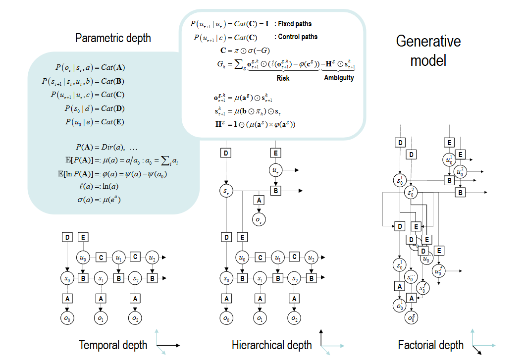
▷ Figure 3. In this study, the generative model—whether applied to decision-making or classification—is represented by two main components: the likelihood, which denotes the probability of an outcome given a cause, and the prior (A). The likelihood quantifies the probability of an outcome occurring for each combination of states (s), while the prior, which depends on random variables, reflects our initial assumptions about the outcome. The prior governing transitions between hidden states (denoted as B) is defined by another prior, and these transitions depend on specific pathways (u), whose probabilities are encoded in C. If certain pathways can minimize the expected free energy (G), then those pathways are more likely to be selected a priori.
Specifically, based on Figure 3, the workflow of the generative model can be outlined as follows:
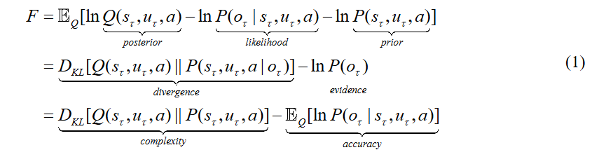
(1) Strategy Selection: The strategy is chosen using a softmax function based on the expected free energy, which in turn determines how subsequent hidden states are generated. During this process, the first term in the final row represents the KL divergence between the approximate posterior distribution (i.e., the state distribution predicted by the model) and the true posterior distribution (i.e., the actual state distribution). This term measures the discrepancy between these distributions, reflecting the model’s complexity (with lower values being preferable). A high complexity may indicate overfitting to the training data, thereby impairing generalization. The second term represents the expected log-likelihood of the observed data under the approximate posterior distribution, which assesses the model’s ability to explain the data. The stronger this explanatory power, the better the model can describe and predict the data, reflecting its accuracy.
(2) Hidden State Generation: A sequence of hidden states is generated according to the probability transitions specified by the chosen combination of pathways. These hidden states represent the model’s internal status at different time points or steps, thereby aiding in the understanding and prediction of data dynamics.
(3) Outcome Generation: The hidden states generate the final outcome through one or more modalities. In this process, the hidden states are inferred from the observed outcome sequence by inverting the generative model. Learning is achieved by updating the model parameters. Notably, the inference process involves setting priors on the (controllable) pathways to minimize the expected free energy.
To facilitate understanding, consider again the example of a tennis match. Here, the first component corresponds to improving the prediction of the opponent’s actions through adjustments to the model parameters; the second component involves constraining the opponent’s choices through one’s own actions; and the third component represents the losses incurred due to observational uncertainty. The active inference model optimizes strategy by minimizing the free energy G(u), thereby gaining a competitive advantage and ultimately achieving victory.

Active Selection and the Renormalization Group
Traditional machine learning methods generally involve using a large dataset to train the model parameters, and then employing these parameters for prediction or classification. However, when the model is excessively complex or the data distribution is too intricate, it becomes necessary to select the most suitable model from among many—one that can handle data both accurately and efficiently.
From the Bayesian perspective, this process is known as “Bayesian model selection.” The parent model, which encompasses all possibilities, can be highly complex and laden with numerous hypotheses. Although many of these hypotheses may be unnecessary, we can eliminate some of them to simplify the model, thereby yielding a child model that is easier to compute and generalize. By comparing how well the parent and child models explain the data—using indicators such as free energy and marginal likelihood—we can determine which model is more parsimonious and powerful. When confronted with new data, this framework enables rapid structural learning by incorporating new latent causes for each unique observation.
During the model selection process, one can compute the difference in expected free energy by comparing the posterior expectations of the parameters under the parent model with those under the augmented model. This difference reflects the information gain achieved by choosing one model over another, capturing the “burden” that the model bears in explaining the data. Based on the magnitude of the log odds ratio, one can decide whether to retain or reject the parent model; this decision is made only when the expected free energy is reduced.
As the dataset grows in scale, the model leverages renormalization group techniques to generate approximate descriptions of fine-scale details at a higher level, thereby efficiently coping with the increased data volume. Take images as an example: one might first view an entire large scene (such as an aerial view of a city), then progressively zoom in on a specific area to examine a street, and finally zoom in further to inspect a particular building. Although the information of interest differs at various scales, these views all pertain to the same scene, with the different scales being interrelated.
The renormalization group capitalizes on this multi-level, multi-scale concept: at each layer, the model simplifies and reprocesses the results from the preceding layer (for instance, by merging certain pixels into a block or by discretizing a continuous speech signal into distinct notes), thereby forming a higher-level, more abstract description. In this way, regardless of how vast the dataset may be, it is progressively “compressed” into simple elements and relationships, significantly reducing the computational burden. Moreover, these higher-level concepts or states can operate across time and space, allowing the model to make effective inferences without getting entangled in every minute detail.
Within the framework of the Renormalizing Generative Model (RGM), this renormalization also extends to the temporal domain: at lower levels, the model might be concerned only with “what happens in the next second,” whereas at higher levels, it is interested in “the overall direction of a scene” or “the theme of the next chapter,” thereby operating over a longer time span. It is akin to watching a movie—one does not focus on every frame, but rather on the overall plot.
In the limit of continuous time, the model’s renormalization can accommodate changes in speed (i.e., acceleration) and even higher-order variations, much like continuous state-space models operating in generalized motion coordinates. From a more intuitive standpoint, sequences encoded at higher levels can be regarded as combinations of events or narrative arcs. In deep hierarchical structures, a single state may generate a sequence of sequences, thereby breaking the Markov property typically seen at the lowest level (where the current state depends only on the immediately preceding state, and not on earlier states). For example, a low-level weather model might focus solely on the relationship between today’s temperature and yesterday’s, while a higher-level model could incorporate the concept of “season” to capture long-term trends.
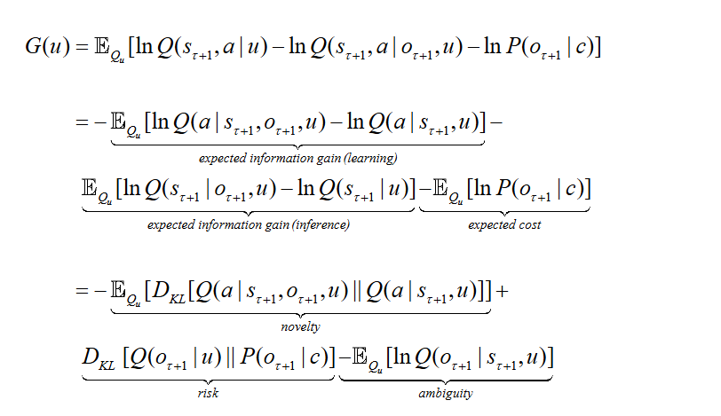
▷ Figure 5. Schematic illustration of the model renormalization process
Additionally, the model undergoes renormalization in its state space. As shown in Figure 5, groups of lower-level states are generated by individual higher-level states, and states at any given level do not share the lower-level substates. This ensures that the latent factors are conditionally independent at each level, allowing for efficient summation and product computations across different layers.
Ultimately, RGM abstracts a complex video, audio, or game scene across multiple temporal and spatial scales. This enables the model to address problems at a more macroscopic level while delegating fine-grained predictions (such as pixel-level changes) to lower-level processes.

Image, Video, and Audio Data Compression and Reconstruction
Renormalizing generative models can be applied to various types of data—including images, video, and audio—for tasks such as classification and recognition. An image consists of continuous pixel values. The model first converts these continuous pixel values into a set of discrete values—a process known as quantization. It then segments the image into small blocks, which can be regarded as “spins.” Through this transformation, the model focuses on processing small regions rather than the entire image; this method is termed the Block-Spin Transformation. Next, singular value decomposition (SVD) is performed to extract the most important information. By discarding insignificant components (i.e., small singular values), the model achieves an initial compression of the image.
This block-based processing and transformation is repeated until a higher level is reached. Each transformation creates a likelihood mapping from higher levels to lower levels—that is, from a global perspective to local details. Then, through Fast Structure Learning, the model learns to generate images based on the structural relationships among different levels. During training, the model recursively applies block transformations to learn the multi-level structure of images while continuously adjusting its parameters to maximize mutual information. Mutual information reflects the amount of useful information that can be extracted from the data; in optimizing the model, the goal is to increase this content as much as possible.
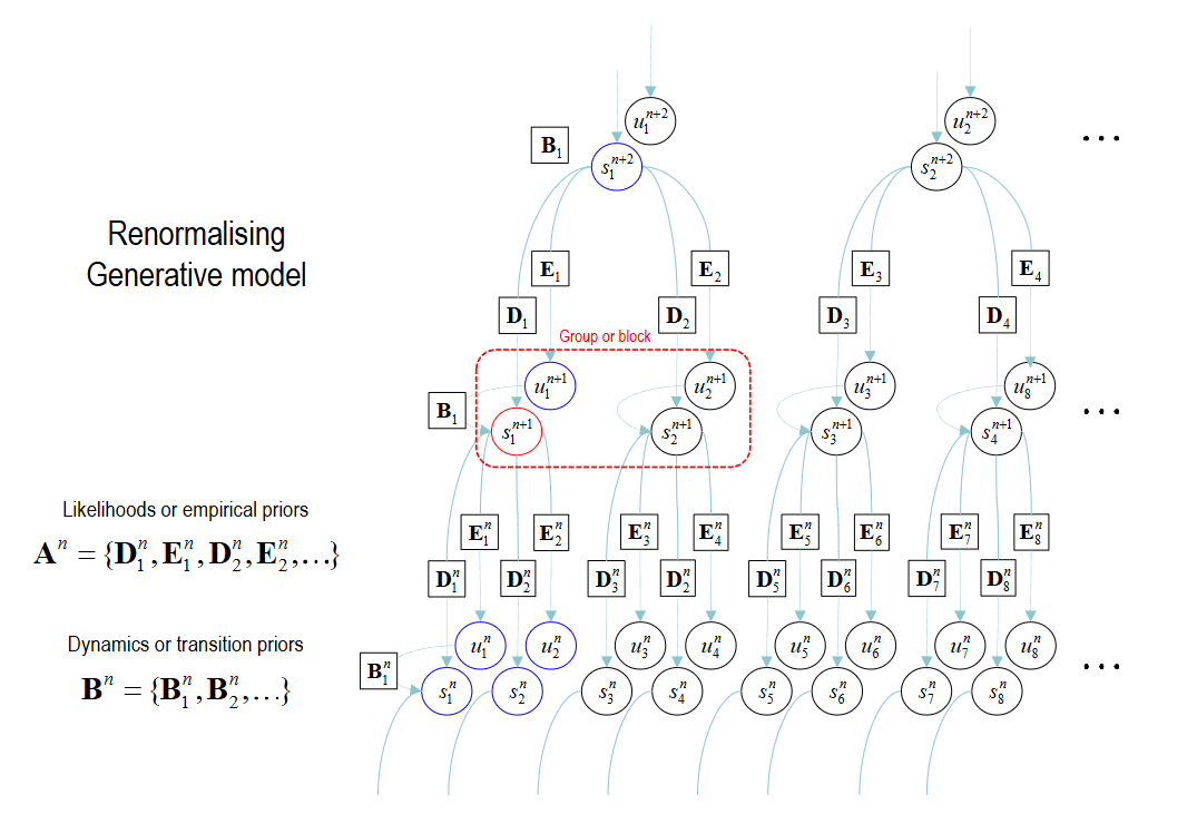
For example, in the MNIST digit classification problem, the model preprocesses the MNIST images and uses a small number of sample images for Fast Structure Learning to generate a renormalizing generative model (RGM) with four levels. Subsequently, the model parameters are optimized via active learning to maximize mutual information.
▷ Figure 6. The quantization process of MNIST images, with the original image on the left and the reconstructed image on the right.
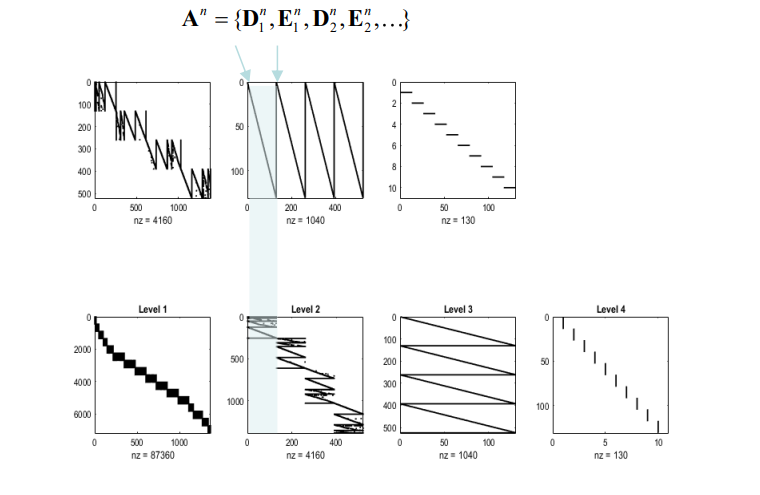
▷ Figure 7. The likelihood mapping in RGM (mapping from one level of the image to another). The top row displays the transposed mapping to illustrate the generative relationship between states at different levels. The renormalizing generative model is applied in the pixel space for object recognition and generation, using a small number of sample images to learn a renormalization structure suitable for lossless compression.
After renormalization, the model generalizes its results through active learning. In other words, during training it optimizes its parameters (for example, the compression method and the selected block transformation) by choosing a subset of data from a large set of images. The model then computes how these images are compressed—via block transformation—to find the most effective compression strategy, ensuring that the compressed images retain as much key information as possible. This active learning ensures a scale-invariant mapping from pixels to objects or digit categories, thereby preserving the mutual information among pixels.
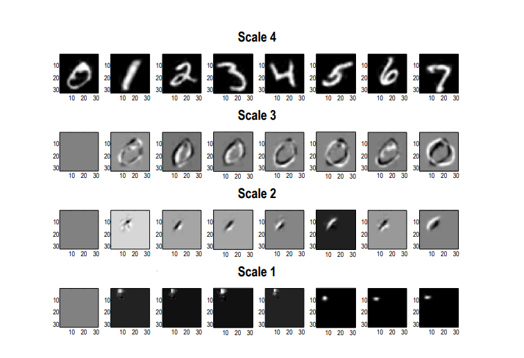
▷ Figure 8. Projection fields of RGM at different levels (the structures learned by the model at various levels). From top to bottom, the levels gradually decrease, with the projection fields shifting from global to local—similar to the progression from simple to complex receptive fields (the image regions that neurons respond to) in the visual system.
In addition to data compression, RGM employs a method to classify test images by predicting the most likely digit category. In active inference, supervision relies on the model’s pre-existing knowledge about the underlying causes of the content, in contrast to traditional learning methods that use class labels as objective functions.
Within active inference, the objective function is a mathematical tool used to assess the “plausibility” or “marginal likelihood” of evidence. By optimizing this function, the model can infer the most likely cause of a phenomenon (e.g., the digit’s category) and determine whether the phenomenon is attributable to a specific cause. In short, the model seeks to find the best explanation by minimizing this objective function, thereby enhancing its accuracy in understanding and inferring the underlying causes of the data.
The aforementioned RGM, after being exposed to 10,000 training images, achieved state-of-the-art classification accuracy on a self-selected subset of test data. Each training image was presented to the model only once in a continuous learning fashion. Importantly, active learning selects only those images that provide the greatest information gain, so the actual number of images used for learning is far fewer than 10,000. This careful selection of data for learning is a recurring theme in later discussions.
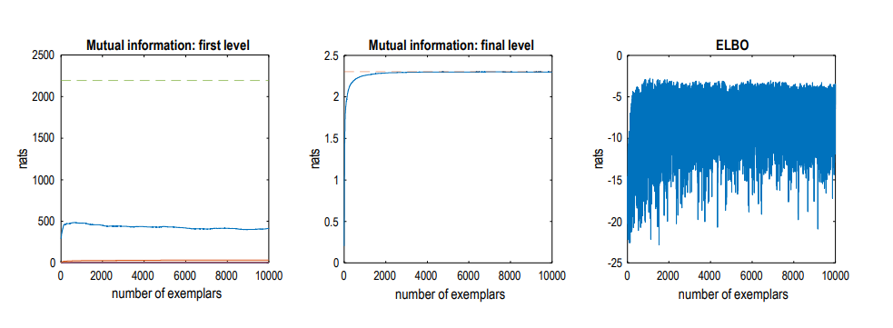
▷ Figure 9. Illustration of the active learning process on the MNIST dataset, including variations in mutual information and variational free energy.
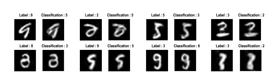
▷ Figure 10. Examples of images misclassified by the RGM model.
The RGM model can also be employed to recognize and generate ordered sequences of images—that is, videos. Specifically, to generate a video, the RGM model takes temporal changes into account by dividing time into different “scales” and applying transformations at each temporal level, ensuring that transitions between frames are both distinct and natural.
Next, the RGM model processes the images by converting spatial (position), color, and temporal information into a standard format—namely, time, color, and pixel voxels—and recording the variations between adjacent voxels. Then, the model segments these processed images into equal-length time intervals. By comparing differences between various time points, it estimates the starting state of each video segment and, based on these estimates, generates a new sequence of time segments. Repeating this process enables the model to construct the overall structure of a video sequence, with each segment’s changes represented by a simple pattern.
For example, in a video of a pigeon flapping its wings, Figure 11 shows the original frames alongside the reconstructed frames after discretization, as well as the process by which RGM generates the film—including posterior predictions of states and paths, and the generated images.
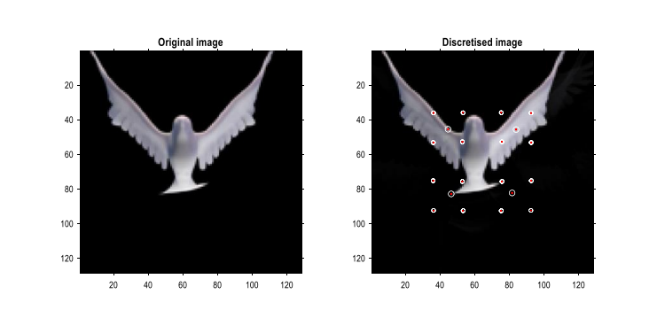
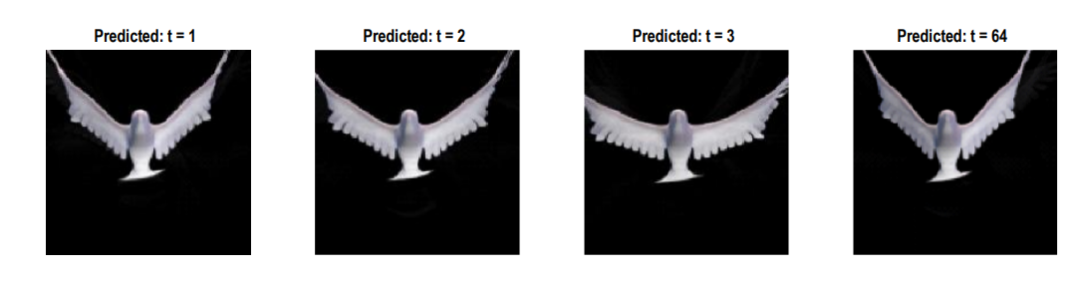
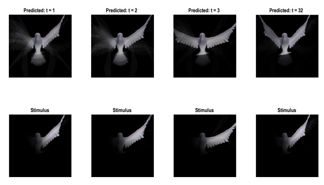
▷ Figure 11. Predicted pigeon flight video generated by the model. Top: An example of how RGM processes an original frame and reconstructs it after discretization, demonstrating that the model can compress high-dimensional data into lower-dimensional representations without losing key information. Middle: How RGM, after learning the video structure, generates new and additional frame sequences through high-level “event sequences,” highlighting the model’s capability not only for reconstruction but also for synthesizing new dynamic content. Bottom: How RGM, when faced with partial (incomplete) input, utilizes its learned statistical structure to infer, complete, and update its prediction of the entire image in real time, showcasing the model’s experience-based prediction and completion ability.
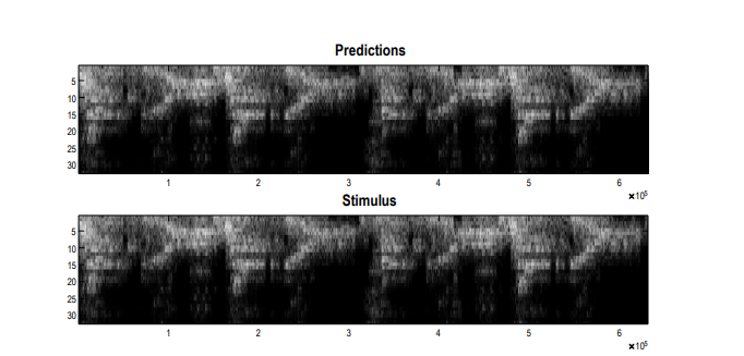
When applying RGM to audio files, pixels are replaced by voxels defined over frequency and time to form a time series. For example, a continuous wavelet transform (CWT) may be used, and its representation can be converted back into an audio signal via an inverse transform for playback. The renormalizing generative model is somewhat simpler for audio than for video, as the data to be processed has only one temporal dimension.
Taking bird calls and jazz music as examples, RGM can compress and reproduce audio. Figure 12 shows the training data for bird calls, including both the continuous wavelet transform and its discrete representation.
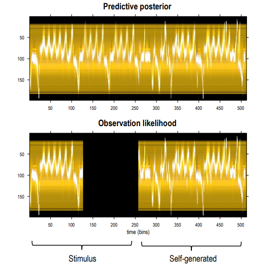
▷ Figure 12. RGM’s renormalization and generation of bird calls, compressing the bird call into a series of events and generating sounds similar to natural bird calls.
▷ Figure 13. Generation of jazz music by RGM, compressing the music into 16 events, with each event corresponding to a musical measure.
▷ Figure 14. Demonstration of RGM’s synchronous prediction ability when provided with an original audio input, analogous to synchronous ensemble performance in music.
RGM can also be applied to planning and inference (reinforcement learning), thereby training agents to make decisions under uncertainty. Within the active inference framework, the decision-making process using RGM is more direct than mere prediction. This process is based on the free energy principle and related theories of embodied cognition. From the perspective of the free energy principle, an agent is viewed as a self-organizing system with characteristic states that describe its type. The existence of an attracting set—which can be described by prior preferences—provides an information-theoretic explanation of how the agent self-organizes.
From a bionic standpoint, RGM does not directly issue motor commands; instead, it controls an agent’s behavior by predicting motion, similar to how humans utilize peripheral reflexes to control bodily actions. This idea stems from the free energy principle’s partitioning of states, where internal and external states are separated through control and sensory channels, leading to active inference— where the control of actions is itself part of the inference process.
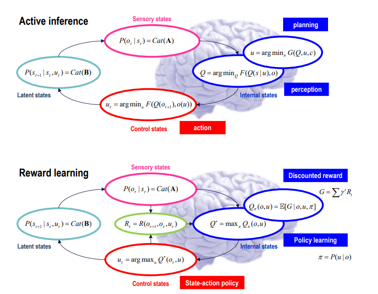
▷ Figure 15. Illustration of the difference between the active inference and reinforcement learning (reward-based learning) paradigms.
Active inference combines control theory with bionics. The fundamental difference between active inference and reinforcement learning is that, in active inference, actions are determined based on posterior predictions of their outcomes—i.e., through Bayesian planning. These predictions arise from policies or plans that minimize expected free energy, thereby illustrating the consequences of actions and reducing uncertainty. In active inference, both belief updating (i.e., perception) and motor control (i.e., action) are processes aimed at minimizing uncertainty. This contrasts sharply with reinforcement learning, where an agent relies on a predefined reward function and updates a mapping between inputs and outputs (from sensory input to control output, typically via deep neural network parameters) through training.
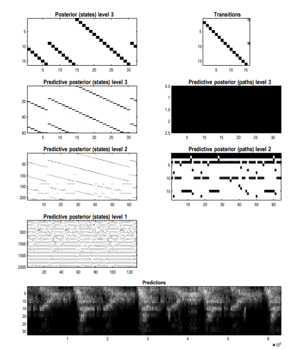
RGM can also be utilized for planning and inference. For instance, in Atari-style games (such as Pong and Breakout), RGM can automatically assemble an agent capable of expert-level gameplay from sequences of outcomes generated by random actions.
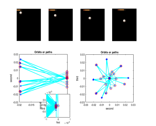
▷ Figure 16. In the application of RGM to the Pong game, this figure shows the resulting paths and trajectories, how the training sequence is compressed, and how transitions between events are managed.

Data “Alchemy”: How Can It Propel the Further Development of AI?
Through the series of experiments and theoretical analyses described above, Friston and his colleagues have demonstrated the remarkable effectiveness of the renormalisation group‐based discrete state‐space model (RGM) across various scenarios. In these applications, model selection, learning, and inversion are achieved by minimising the expected free energy. Because active inference methods are grounded in the free energy principle, employing the renormalisation group becomes relatively straightforward, effectively addressing the challenges of large‐scale data processing. Moreover, the free energy principle itself is a scale‐invariant variational principle, naturally suited to systems operating at different scales.
Thus, RGM holds tremendous potential across multiple domains. For instance, in image and video processing, it can enable more efficient compression and generation, thereby saving storage space and improving data transmission efficiency. In audio processing, the ability to effectively compress and generate sound is crucial for storage and transmission. It also offers fresh perspectives for music creation and sound recognition. In gaming and planning, the model can help agents learn expert strategies to achieve smarter decision‐making and actions, thereby advancing artificial intelligence applications in gaming, robotic control, and other decision‐making tasks.
The RGM features a simple structure and high efficiency, allowing it to rapidly learn its own architecture. However, it may not yet be ideally suited for modelling highly complex systems. Future research could explore converting continuous state‐space models into discrete ones and employing renormalisation procedures for learning, along with improving model parameterisation to suit a wider range of applications. More broadly, this renormalisation group‐based approach provides a novel framework for understanding and managing complex systems, shedding light on the ubiquitous scale invariance and principles of structural learning in nature while offering insights for research in physics, biology, and computer science.
The vast majority of existing artificial intelligence systems rely on enormous amounts of data; the efficiency with which these systems learn from and leverage data determines their problem‐solving capabilities. Historically, ancient alchemy spurred the development of metallurgy, enabling us to refine and utilise metals more effectively. Today, we are similarly attempting to treat raw, unprocessed data as a “raw material” from which deep structures, regularities, and patterns can be extracted to uncover valuable insights. Perhaps in the near future, AI with enhanced data processing capabilities will be able to provide decision support as robust as Moss in The Wandering Earth, becoming an indispensable assistant in deducing optimal solutions to complex problems.